Statistic and Probability
Data types
Discrete Data: - integer based, often counts of some event. - How many purchases did a customer make in a yera? - How many times did I flif heads? Continous Data - Has an infinite number of possible values - How much time did it take for a user to check out? - How much rain fell on a givern day?
Categorical Data: Qualitative data - Gender, Yes/ no, race, etc.
Ordinal: A miture of numerical and categorical - Categorical data that has mathematical meaning: 1 means worse movie than a 2

Mode: the most common number in a data set
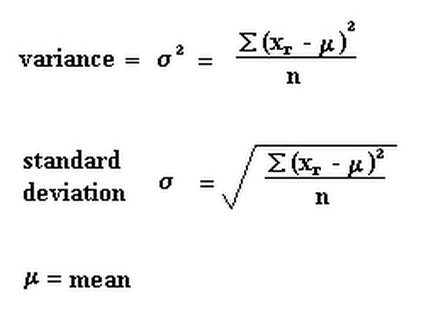
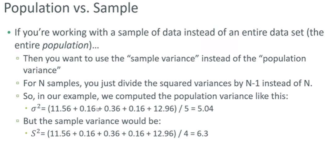
Variance:
Measeures how “pread-out” the data is. Variance is the average of the squared differences from the mean EXAMPLE: Variance of set (1, 4, 5, 4, 8) - First find the mean (1+4+5+4+8)/5 = 4.4 = Now find the differences from the mean: (1 - 4.4, 4- 4.4, 5 - 4.4, etc) - (-3.4, -0.4, 0.6, -0.4, 3.6) - find the squared differences: (11.56, 0.16, 0.36, 0.16, 12.96) - find the average of the squared differences: a~2 = (11.56 + 0.16 + 0.36 + 0.16 + 12.96) / 5 = 5.04
Standard deviation:
Square room of the variance
Is usually used as a way to identify outliers (wartości odstajace). Data points that lie more than one standard deviation from the mean can be considered unusual.
You can talk about how extreme a data point is by talking about “how many sigmas” away from the mean iti is.
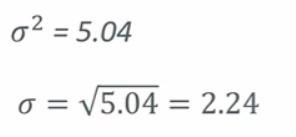
So, the standard variation of (1, 4, 5, 4, 8) is 2.24.
import numpy as np
import matplotlib.pyplot as plt

income = np.random.normal(100, 20.0, 10000)

plt.hist(income, 50)
plt.show()
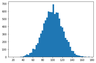
income.std()
20.052036933618258
income.var()
402.0841851871907
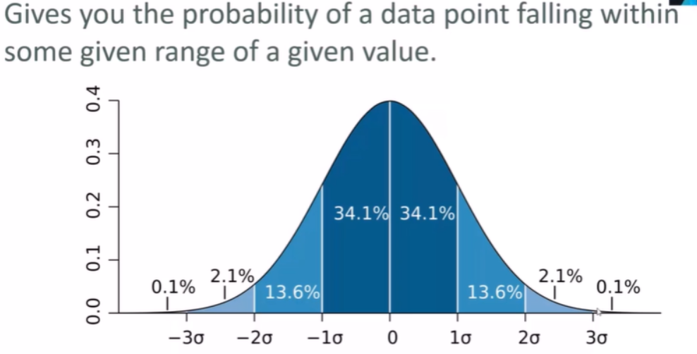
Normal distribution:
Gives you the probability of a data point falling within some given range of a given value
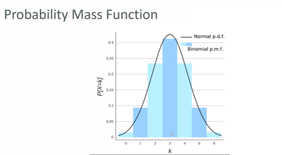
Probability Mass Function:
The way we viualise the probbility of discreet data occurring
Examples of Data Distributions
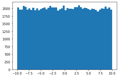
Uniform Distribution
values = np.random.uniform(-10., 10., 100000)
plt.hist(values, 50)
plt.show()
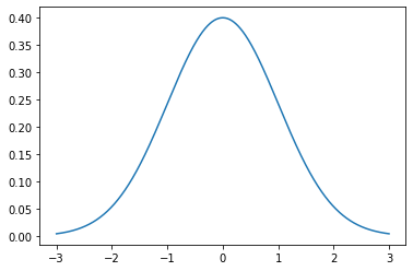
Normal / Gaussian
from scipy.stats import norm

x = np.arange(-3, 3, 0.001)
plt.plot(x, norm.pdf(x)) # pdf probability density function
plt.show()
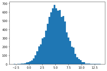
Generate some random numbers with a normal distribution. “mu” is the desired mean, “sigma” is the standard deviation.
mu = 5.1
sigma = 2.0
values = np.random.normal(mu, sigma, 10000)
plt.hist(values, 50)
plt.show()
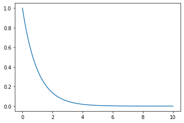
Exponential PDF / “Power Law”
from scipy.stats import expon

x = np.arange(0, 10, 0.001)
plt.plot(x, expon.pdf(x))
plt.show()
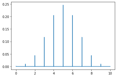
Binomial Probability Mass Function
from scipy.stats import binom

n, p = 10, 0.5
x = np.arange(0, 10, 0.001)
plt.plot(x, binom.pmf(x, n, p))
plt.show()
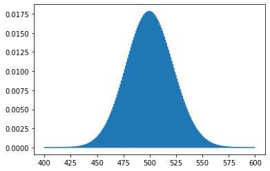
Poisson Probability Mass Funtion
My website gets on average 500 visits per day, what’s the odds of getting 550?
from scipy.stats import poisson

mu = 500
x = np.arange(400, 600, 0.5)
plt.plot(x, poisson.pmf(x, mu))
plt.show()
Moments
Quantitative measures of the shape of a probability density function
Mathematically they are hard to wrap up:

- The first moment is the mean.
- The second moment is the variance.
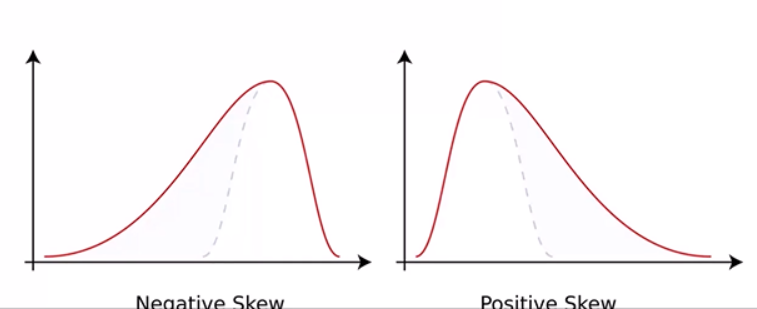
- Third moment is “skew”
- How loopsided is the distribution?
- A distribution with a longer tail on the left will be skewed left, and have a negative skew.
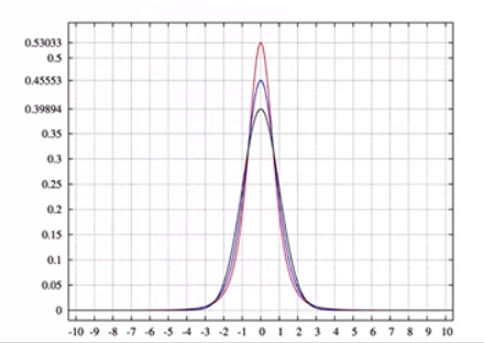
- The fourth moment is “kurtosis”
- How thick is the tail, and how sharp is the peak, compared to a normal distribution?
- F. e.: higher peaks have highter kurtosis
import numpy as np
import matplotlib.pyplot as plt

vals = np.random.normal(0, 0.5, 10000)

plt.hist(vals, 50)
plt.show()
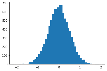
# FIRST MOMENT: MEAN - data should be close to 0
np.mean(vals)
0.0008176312786928964
# SECOND MOMENT: VARIANCE
np.var(vals)
0.25131555488252116
# THIRD MOMENT: SKEW - data is nicely centered around 0, it should be almost 0
import scipy.stats as sp
sp.skew(vals)
-0.03052643631658173
# FOURTH MOMENT: KURTOSIS - describes the shape of the tail. For a normal distribution, this is 0
sp.kurtosis(vals)
0.0302581860757547
Covariance
Measures how two variables vary in tandem from their means.
- think of the data sets for the two variables as high-dimensional vetors
- convert these to vectors of variances from the mean
- take the dot product (cosine of the angle between them) of the two vectors
- divide by the sample size
Correlation
Just divide the covariance by the stanard deviations of both variables, and that normalizes things
- so a correlation of -1 means a perfect inverse correlation
- correlation of 0: no correlation
- correlation 1: perfect correlation
def de_mean(x):
    xmean = np.mean(x)
    return [xi - xmean for xi in x]

def covariance(x, y):
    n = len(x)
    return np.dot(de_mean(x), de_mean(y)) / (n-1)
pageSpeed = np.random.normal(3.0, 1.0, 1000)
purchaseAmount = np.random.normal(50.0, 10.0, 1000)

plt.scatter(pageSpeed, purchaseAmount)
plt.show()
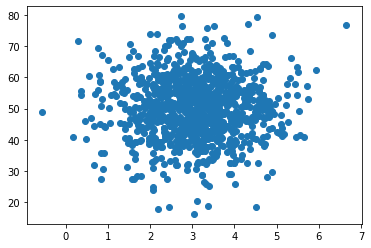
covariance(pageSpeed, purchaseAmount)
0.015213838310440675
purchaseAmount = np.random.normal(50.0, 10.0, 1000) / pageSpeed

plt.scatter(pageSpeed, purchaseAmount)
plt.show()
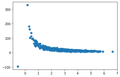
covariance(pageSpeed, purchaseAmount)
-9.760127236964708
def correlation(x,y ):
    stddevx = x.std()
    stddevy = y.std()
    return covariance(x, y) / stddevx / stddevy
correlation(pageSpeed, purchaseAmount)
-0.5682282401242628
np.corrcoef(pageSpeed, purchaseAmount)
array([[ 1.        , -0.56766001],
       [-0.56766001,  1.        ]])
purchaseAmount = 100 - pageSpeed * 3

plt.scatter(pageSpeed, purchaseAmount)
plt.show()
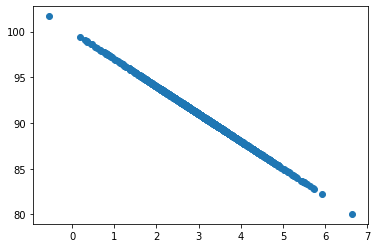
correlation(pageSpeed, purchaseAmount)
-1.001001001001001
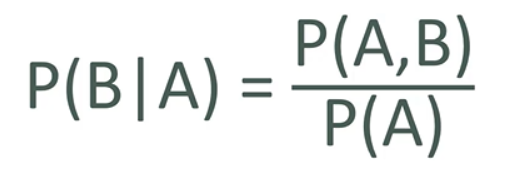
Conditional Probability
- If I have two events that depend on each other, what’s the probability that both will occur?
- Notation: P(A, B) is the probability of A and B both occuring
-
P(B A): Probability of B given that A has occurred
EXAMPLE: I give my student two tests.
60% of my students passed bth tests, but the first test was easier - 80% passed that one.

What percentage of students who passed the first test also passed the second?
A = passing the firt test, B = passing the second test
| So we are asking for P(B | A) - the probability of B given A |
| P(B | A) = P(A, B) / P(A) = 0.6 / 0.8 = 0.75 |
ANSWER: 75% of students who passed the first test passed the second
totals = {20:0, 30:0, 40:0, 50:0, 60:0, 70:0}
purchases = {20:0, 30:0, 40:0, 50:0, 60:0, 70:0}
totalPurchases = 0

for _ in range(100000):
    ageDecade = np.random.choice([20, 30, 40, 50, 60, 70])
    purchaseProbability = float(ageDecade) / 100.0
    totals[ageDecade] += 1
    if np.random.random() < purchaseProbability:
        totalPurchases += 1
        purchases[ageDecade] += 1
totals
{20: 16593, 30: 16697, 40: 16526, 50: 16659, 60: 16808, 70: 16717}
purchases
{20: 3372, 30: 4987, 40: 6652, 50: 8284, 60: 10125, 70: 11699}
totalPurchases
45119
| First let’s compute P(E | F) |
E = purchase
F = “you’re in your 30’s”
The probability of someone in their 30’s buying something is just the percentage of how many 30 y.o. bought something
PEF = float(purchases[30] / totals[30])
PEF
0.29867640893573694
P(F) is a probability of being 30 in this dataset:
PF = totals[30] / 100_000
PF
0.16697
PE is the overall probability of buing something
PE = totalPurchases / 100_000
PE
0.45119
| If E and F were independent, then we would expect P(E | F) to be about the same as P(E). |
But they are not.
| P(E, F) is different from P(E | F). |
P(E, F) would be the probability of both being in your 30’s and buing something out of the total population - not just the people in their 30s
PEF2 = purchases[30] / 100_000
PEF2
0.04987
Product of P(E) and P(F), P(E)P(F)
PF * PE
0.0753351943
Sometimg you may learn in statics is that P(E, F) = P(E)P(F)
But this assumes E and F are independent.
We’ve found that P(E, F) is about 0.5 while P(E)P(F) is about 0.75.
So when E and F are dependent and we hava a conditional probability going on, we can;t just say that P(E, F) = P(E)P(F)
| We can also check that P(E | F) = P(E, F) / P(F) |
(purchases[30] / 100_000) / PF
0.29867640893573694
totals = {20:0, 30:0, 40:0, 50:0, 60:0, 70:0}
purchases = {20:0, 30:0, 40:0, 50:0, 60:0, 70:0}
totalPurchases = 0

for _ in range(100000):
    ageDecade = np.random.choice([20, 30, 40, 50, 60, 70])
    purchaseProbability = 0.4
    totals[ageDecade] += 1
    if np.random.random() < purchaseProbability:
        totalPurchases += 1
        purchases[ageDecade] += 1
purchases[70] / totalPurchases
0.16670408341440296
purchases[70] / totals[70]
0.4003234695100036
purchases[20] / totalPurchases
0.16717802888572925
purchases[20] / totals[20]
0.4009332376166547
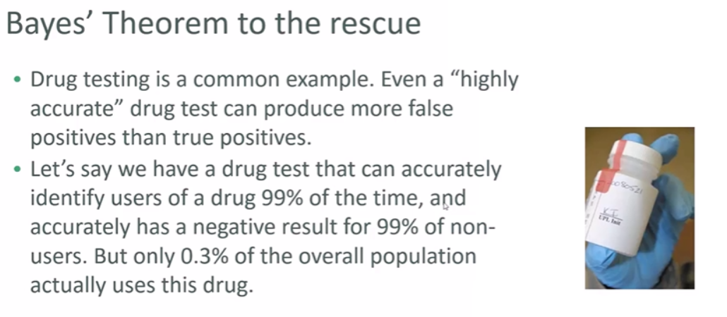
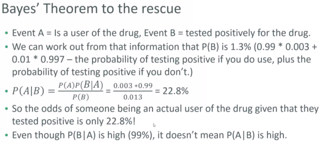
Bayes’ Theorem
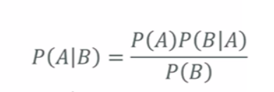
The probability of A given B, is the probability of A times the probability of B given A ver the probability of B.
Prawdopodobieństwo A danego B jest prawdopodobieństwem A razy prawdopodobieństwo B przy danym A w stosunku do prawdopodobieństwa B.
The key insight is that the probability of something that depends on B depends very much on the base probability of A and B.