Predictive Models - Regression
Linear Regression
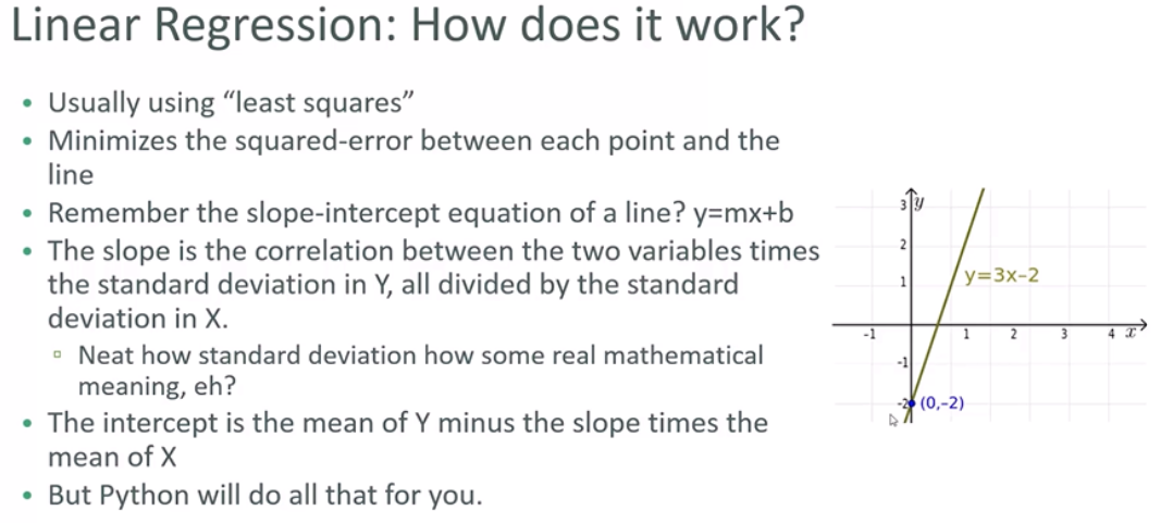
Least squares minimizes the sum of squared errors
This is the same as maximizing the likelihood of observed data if you start thinking of the problem in terms of probabilities and probability distribution functions
Sometimes called “maximum likelihood estimation”
import numpy as np
import matplotlib.pyplot as plt
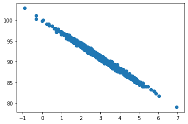
pageSpeed = np.random.normal(3.0, 1.0, 1000)
purchaseAmount = 100 - (pageSpeed + np.random.normal(0, 0.1, 1000)) * 3
plt.scatter(pageSpeed, purchaseAmount)
plt.show()
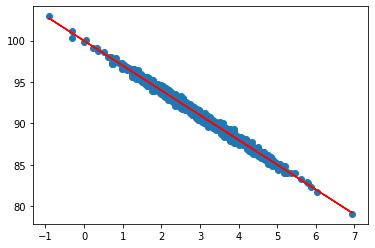
from scipy import stats

slope, intercept, r_value, p_value, std_err = stats.linregress(pageSpeed, purchaseAmount)
R squared value shows a really good fit
r_value ** 2
0.9902693736994506
def predict(x):
    return slope * x + intercept

fitline = predict(pageSpeed)

plt.scatter(pageSpeed, purchaseAmount)
plt.plot(pageSpeed, fitline, c="r")
plt.show()
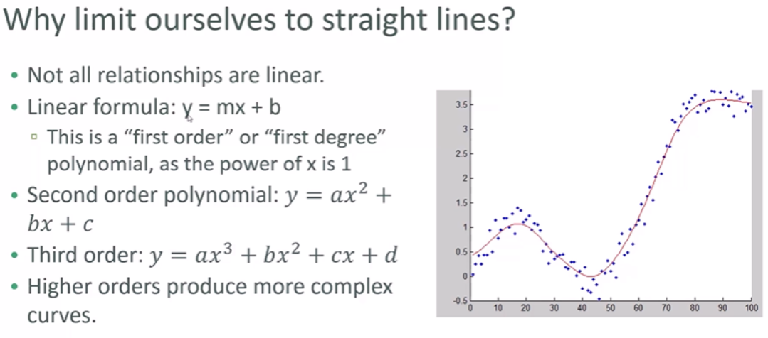
Polynomial Regression
np.random.seed(2020)

pageSpeed = np.random.normal(3.0, 1.0, 1000)
purchaseAmount = np.random.normal(50.0, 10.0, 1000) / pageSpeed

plt.scatter(pageSpeed, purchaseAmount)
plt.show()
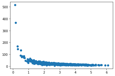
x = np.array(pageSpeed)
y = np.array(purchaseAmount)

p4 = np.poly1d(np.polyfit(x, y, 4))
p4
poly1d([   2.43355681,  -33.88400278,  168.02869346, -354.05850288,
        286.61089763])
xp = np.linspace(0, 7, 100)
plt.scatter(x, y)
plt.plot(xp, p4(xp), c="r")
plt.show()
from sklearn.metrics import r2_score

r2 = r2_score(y, p4(x))
r2
0.6980067595161712
Multiple regression
import pandas as pd

df = pd.read_excel("http://cdn.sundog-soft.com/Udemy/DataScience/cars.xls")
df.head()
| Price | Mileage | Make | Model | Trim | Type | Cylinder | Liter | Doors | Cruise | Sound | Leather | |
|---|---|---|---|---|---|---|---|---|---|---|---|---|
| 0 | 17314.103129 | 8221 | Buick | Century | Sedan 4D | Sedan | 6 | 3.1 | 4 | 1 | 1 | 1 |
| 1 | 17542.036083 | 9135 | Buick | Century | Sedan 4D | Sedan | 6 | 3.1 | 4 | 1 | 1 | 0 |
| 2 | 16218.847862 | 13196 | Buick | Century | Sedan 4D | Sedan | 6 | 3.1 | 4 | 1 | 1 | 0 |
| 3 | 16336.913140 | 16342 | Buick | Century | Sedan 4D | Sedan | 6 | 3.1 | 4 | 1 | 0 | 0 |
| 4 | 16339.170324 | 19832 | Buick | Century | Sedan 4D | Sedan | 6 | 3.1 | 4 | 1 | 0 | 1 |
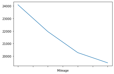
df1 = df[["Mileage", "Price"]]

bins = np.arange(0, 50000, 10000)
groups = df1.groupby(pd.cut(df1["Mileage"], bins)).mean()
groups.head()
| Mileage | Price | |
|---|---|---|
| Mileage | ||
| (0, 10000] | 5588.629630 | 24096.714451 |
| (10000, 20000] | 15898.496183 | 21955.979607 |
| (20000, 30000] | 24114.407104 | 20278.606252 |
| (30000, 40000] | 33610.338710 | 19463.670267 |
groups["Price"].plot.line()
<matplotlib.axes._subplots.AxesSubplot at 0x292b9325488>
import statsmodels.api as sm
from sklearn.preprocessing import StandardScaler

scale = StandardScaler()
X = df[["Mileage", "Cylinder", "Doors"]]
y = df["Price"]
X[["Mileage", "Cylinder", "Doors"]] = scale.fit_transform(
    X[["Mileage", "Cylinder", "Doors"]])
R:\Work\Anacond\lib\site-packages\ipykernel_launcher.py:2: SettingWithCopyWarning:
A value is trying to be set on a copy of a slice from a DataFrame.
Try using .loc[row_indexer,col_indexer] = value instead

See the caveats in the documentation: https://pandas.pydata.org/pandas-docs/stable/user_guide/indexing.html#returning-a-view-versus-a-copy

R:\Work\Anacond\lib\site-packages\pandas\core\indexing.py:965: SettingWithCopyWarning:
A value is trying to be set on a copy of a slice from a DataFrame.
Try using .loc[row_indexer,col_indexer] = value instead

See the caveats in the documentation: https://pandas.pydata.org/pandas-docs/stable/user_guide/indexing.html#returning-a-view-versus-a-copy
  self.obj[item] = s
X
| Mileage | Cylinder | Doors | |
|---|---|---|---|
| 0 | -1.417485 | 0.52741 | 0.556279 |
| 1 | -1.305902 | 0.52741 | 0.556279 |
| 2 | -0.810128 | 0.52741 | 0.556279 |
| 3 | -0.426058 | 0.52741 | 0.556279 |
| 4 | 0.000008 | 0.52741 | 0.556279 |
| ... | ... | ... | ... |
| 799 | -0.439853 | 0.52741 | 0.556279 |
| 800 | -0.089966 | 0.52741 | 0.556279 |
| 801 | 0.079605 | 0.52741 | 0.556279 |
| 802 | 0.750446 | 0.52741 | 0.556279 |
| 803 | 1.932565 | 0.52741 | 0.556279 |
804 rows × 3 columns
est = sm.OLS(y, X).fit()
est.summary()
| Dep. Variable: | Price | R-squared (uncentered): | 0.064 |
|---|---|---|---|
| Model: | OLS | Adj. R-squared (uncentered): | 0.060 |
| Method: | Least Squares | F-statistic: | 18.11 |
| Date: | Wed, 28 Oct 2020 | Prob (F-statistic): | 2.23e-11 |
| Time: | 14:40:09 | Log-Likelihood: | -9207.1 |
| No. Observations: | 804 | AIC: | 1.842e+04 |
| Df Residuals: | 801 | BIC: | 1.843e+04 |
| Df Model: | 3 | ||
| Covariance Type: | nonrobust |
| coef | std err | t | P>|t| | [0.025 | 0.975] | |
|---|---|---|---|---|---|---|
| Mileage | -1272.3412 | 804.623 | -1.581 | 0.114 | -2851.759 | 307.077 |
| Cylinder | 5587.4472 | 804.509 | 6.945 | 0.000 | 4008.252 | 7166.642 |
| Doors | -1404.5513 | 804.275 | -1.746 | 0.081 | -2983.288 | 174.185 |
| Omnibus: | 157.913 | Durbin-Watson: | 0.008 |
|---|---|---|---|
| Prob(Omnibus): | 0.000 | Jarque-Bera (JB): | 257.529 |
| Skew: | 1.278 | Prob(JB): | 1.20e-56 |
| Kurtosis: | 4.074 | Cond. No. | 1.03 |
Warnings:
[1] Standard Errors assume that the covariance matrix of the errors is correctly specified.
y.groupby(df.Doors).mean()
Doors
2    23807.135520
4    20580.670749
Name: Price, dtype: float64
Surprisingly more doors doesn’t mean higher price.
So it’s pretty useless as a predictor here.
scaled = scale.transform([[45000, 8, 4]])
predicted = est.predict(scaled[0])
scaled, predicted
(array([[3.07256589, 1.96971667, 0.55627894]]), array([6315.01330583]))
Multi-Level Models