Machine Learning with Python, Part 2

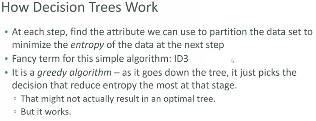
Decision Tree

import numpy as no
import pandas as pd
from sklearn import tree

df = pd.read_csv("data/PastHires.csv")
df.head()

	Years Experience	Employed?	Previous employers	Level of Education	Top-tier school	Interned	Hired
0	10	Y	4	BS	N	N	Y
1	0	N	0	BS	Y	Y	Y
2	7	N	6	BS	N	N	N
3	2	Y	1	MS	Y	N	Y
4	20	N	2	PhD	Y	N	N

d = {"Y":1, "N":0}
df["Hired"] = df["Hired"].map(d)
df["Hired"]

   1
   1
   0
   1
   0
   1
   1
   1
   1
   0
  0
  1
  1
Name: Hired, dtype: int64

df["Employed?"] = df["Employed?"].map(d)
df["Top-tier school"] = df["Top-tier school"].map(d)
df["Interned"] = df["Interned"].map(d)

d = {"BS":0, "MS":1, "PhD":2}
df["Level of Education"] = df["Level of Education"].map(d)

df.head()

	Years Experience	Employed?	Previous employers	Level of Education	Top-tier school	Interned	Hired
0	10	1	4	0	0	0	1
1	0	0	0	0	1	1	1
2	7	0	6	0	0	0	0
3	2	1	1	1	1	0	1
4	20	0	2	2	1	0	0

features = list(df.columns[:6])
features

['Years Experience',
 'Employed?',
 'Previous employers',
 'Level of Education',
 'Top-tier school',
 'Interned']

y = df["Hired"]
X = df[features]

clf = tree.DecisionTreeClassifier()
clf = clf.fit(X, y)

from IPython.display import Image
from sklearn.externals.six import StringIO
import pydotplus as pydot

# !pip install pydotplus

# dot_data = StringIO()
# tree.export_graphviz(clf, out_file=dot_data, feature_names=features)
# graph = pydot.graph_from_dot_data(dot_data.getvalue())
# Image(graph.create_png())

from sklearn.ensemble import RandomForestClassifier
import numpy as np

clf = RandomForestClassifier(n_estimators = 10)
clf = clf.fit(X, y)

clf.predict(np.array([10, 1, 4, 0, 0, 0]).reshape(1, -1))

array([1], dtype=int64)

clf.predict(np.array([10, 0, 4, 0, 0, 0]).reshape(1, -1))

array([0], dtype=int64)

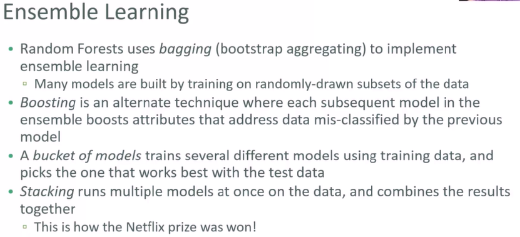
Ensemble Learning

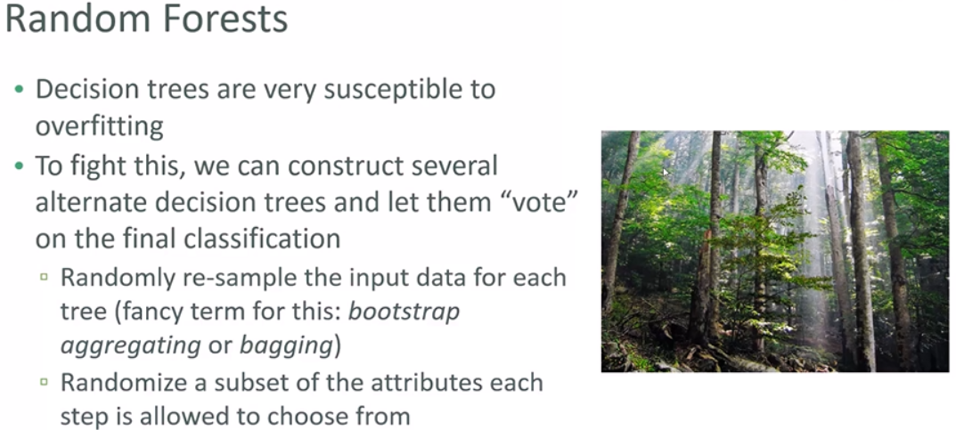
Random Forests was an example of ensemble learning.

It just means we use models to try and solve the same roblem, and let them vote on the results.

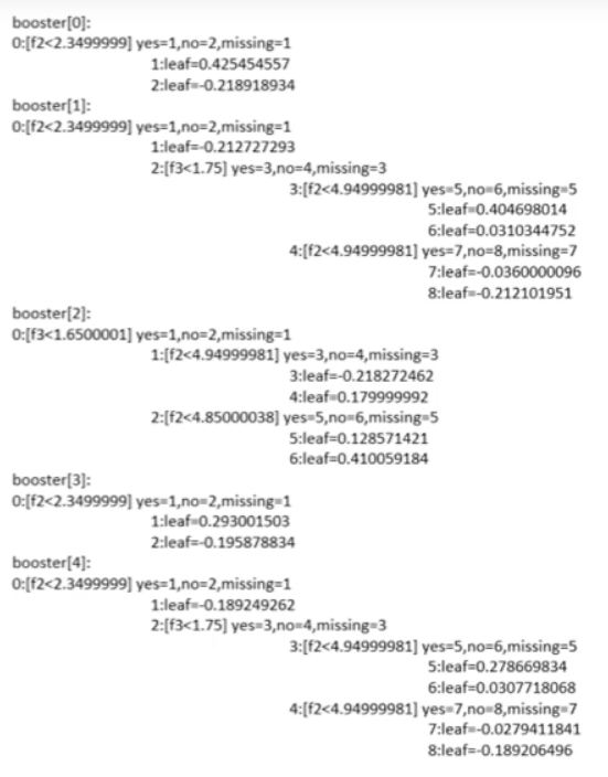
CGBoost

eXtreme Gradient Boosted Trees

Remember, boosting is an ensemble method - each tree boosts attributes that let to misclassifications of previous tree

More facts: - routinely winds Kaggle competitions - easy to use and fast

from sklearn.datasets import load_iris

iris = load_iris()

numSamples, numFeatures = iris.data.shape

numSamples, numFeatures

(150, 4)

iris.target_names

array(['setosa', 'versicolor', 'virginica'], dtype='<U10')

from sklearn.model_selection import train_test_split

X_train, X_test, Y_train, Y_test = train_test_split(
    iris.data, iris.target, test_size=0.2, random_state=1)
# with random_state=0, the accuracy_score is equal 1.0

import xgboost as xgb

train = xgb.DMatrix(X_train, label=Y_train)
test = xgb.DMatrix(X_test, label=Y_test)

param = {
    "max_depth":3,
    "eta":0.3,
    "objective":"multi:softmax",
    "num_class":3
}

epochs=10

model = xgb.train(param, train, epochs)

predictions = model.predict(test)
predictions

array([0., 1., 1., 0., 2., 1., 2., 0., 0., 2., 1., 0., 2., 1., 1., 0., 1.,
       1., 0., 0., 1., 1., 2., 0., 2., 1., 0., 0., 1., 2.], dtype=float32)

from sklearn.metrics import accuracy_score

accuracy_score(Y_test, predictions)

0.9666666666666667

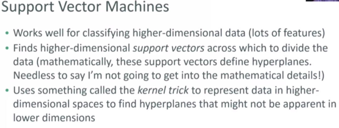
Support Vector Machines

The important point is that SVM’s employ some advanced mathematical trickery to cluster data, and it can handle datasets with lots of features.

It’s also fairly expensive - the “kernel trick” is the only thing that makes it possible.

def createClusteredData(N, k):
    np.random.seed(2020)
    pointsPerCluster = float(N)/k
    X, y = [], []
    for i in range(k):
        incomeCentroid = np.random.uniform(2000., 200000.)
        ageCentroid = np.random.uniform(20.0, 70.)
        for j in range(int(pointsPerCluster)):
            X.append([np.random.normal(incomeCentroid, 10000.), 
                      np.random.normal(ageCentroid, 2.0)])
            y.append(i)
    X = np.array(X)
    y = np.array(y)
    return X, y

from pylab import *
from sklearn.preprocessing import MinMaxScaler

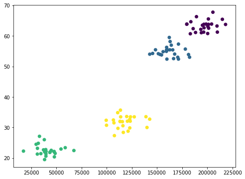
(X, y) = createClusteredData(100, 4)

plt.figure(figsize=(8, 6))
plt.scatter(X[:, 0], X[:, 1], c=y.astype(np.float))
plt.show()

png

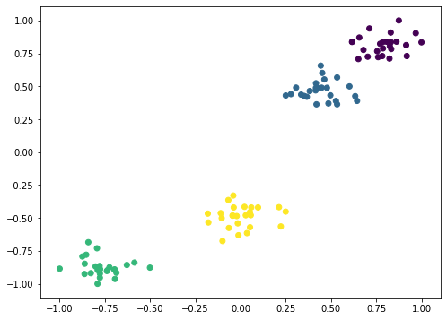
scaling = MinMaxScaler(feature_range=(-1, 1)).fit(X)
X = scaling.transform(X)

plt.figure(figsize=(8, 6))
plt.scatter(X[:, 0], X[:, 1], c=y.astype(np.float))
plt.show()

png

from sklearn import svm, datasets

C = 1.0
svc = svm.SVC(kernel="linear", C=C).fit(X, y)

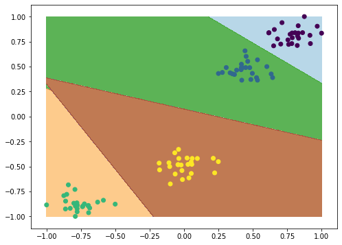
def plotPredictions(clf):
    # create a dense grid of points to sample
    xx, yy = np.meshgrid(np.arange(-1, 1, .001),
                        np.arange(-1, 1, .001))
    # convert to Numpy arrays
    npx = xx.ravel()
    npy = yy.ravel()
    
    # convert to aa list of 2D (income, age) points
    samplePoints = np.c_[npx, npy]
    
    # Generte predicted labels (cluster numbers) for each point
    Z = clf.predict(samplePoints)
    
    plt.figure(figsize=(8, 6))
    Z = Z.reshape(xx.shape) # reshape results to match xx dimension
    plt.contourf(xx, yy, Z, cmap=plt.cm.Paired, alpha=0.8) # draw the contour
    plt.scatter(X[:, 0], X[:, 1], c=y.astype(np.float))
    plt.show()

plotPredictions(svc)

png

svc.predict(scaling.transform([[20000, 40]]))

array([2])

svc.predict(scaling.transform([[5000, 65]]))

array([1])