Classification and Representation

Classification
To attempt classification, one method is to use linear regression and map all predictions greater than $0.5$ as a $1$, and all less than $0.5$ as a $0$. However, this method doesn’t work well because classification is not actually a linear function.
The classificaion problem is just like the regression problem, except that the values we now want to predict take on only a small number of discrete values.
For now, we will focus on the binary classification problem in which $y$ can take only two values, $0$ and $1$. (Most of what we say here will also generalize to the multiple-class case.)
For instance, if we are trying to build spam classifier for email, then $x^{(i)}$ may be some features of a piece of email, and $y$ may be $1$ if it is a piece of spam mail, and $0$ otherwise.
Hence $y \in { 0, 1 }$. $0$ is also called the negative class, and $1$ the positive class, and they are sometimes also denoted by the symbols “-“ and “+”. Given $x^{(i)}$, the corresponding $y^{(i)}$ is also called the label for the training example.
Hypothesis Representation
We could approach the classification problem ignoring the fact that $y$ is discrete-values, and use our old linear regression algorithm to try to predict $y$ given $x$. However, it is easy to construct examples where this method performs very poorly. Intuitively, it also doesn’t make sense for $h_{\theta}(x)$ to take values larger than $1$ or smaller than $0$ when we know that $y \in { 0, 1 }$.
To fix this, let’s change the form for our hypothesis $h_{\theta}(x)$ to satisfy $0 \ge h_{\theta}(x) \ge 1$. This is accomplished by plugging $\theta^Tx$ into the Logistic Function.
Our new form uses the Sigmoid Function, also called the Logistic Function:
The following image shows us what the sigmoid function looks like:
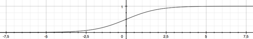
The function $g(z)$ shown here maps any real number to the $(0, 1)$ interval, making it useful for transforming an arbitrary-values function into a function better suited for classification.
$h_{\theta}(x)$ will give us the probability that our input is $1$.
For example, $h_{\theta}(x) = 0.7$ gives us a probability of %70%% that our output is $1$. Our probability that our prediction is $0$ is just the complement of our probability that it is 1 (e.g, if probability that it is $1$ is $70\%$, then the probability that it is $0$ is $30\%$).
Decision Boundary
In order to get our discrete $0$ or $1$ classification, we can translate the output of the hypothesis function as follows:
The way our logistic function $g$ behaves is that when its output is greater than or equal to zero, its output is greater than or equal $0.5$:
Remember:
So if our input to $g$ is $\theta^TX$, then that means:
From these statements we can now say:
The decision boundary is the line that separates the area where $y = 0$ and where $y = 1$. It is created by our hypothesis function.
Example:
In this case, our decision boundary is a straight vertical line placed on the graph, where x_1 = 5, and everything to the left of that denotes $y = 1$, while everything to the right denotes $y = 0$.
Again, the input to the sigmoid function $g(z)$ (e.g. $\theta^TX$ deosn’t need to be linear, and could be a function that describes a circle (e.g. $z = \theta_0 + \theta_1x_1^2 + \theta_2x_2^2 $ or any shape to fit our data.